Connect code and reports with

Typical guidelines for keeping a notebook of wet-lab work

1. Record everything you do in the lab, even if you are following a published procedure.
2. If you make a mistake, put a line through the mistake and write the new information next to it.
3. Use a ball point pen so that marks will not smear nor will they be erasable.
4. Use a bound notebook so that tear-out would be visible.
5. When you finish a page, put a corner-to corner line through any blank parts that could still be used for data entry.
6. All pages must be pre-numbered.
7. Write a title for each and every new set of entries.
8. It is critical that you enter all procedures and data directly into your notebook in a timely manner.
9. Properly introduce and summarize each experiment.
10. The investigator and supervisor must sign each page.

etc...

Typical guidelines for keeping a notebook of dry-lab work

Literate programming

Instead of imagining that our main task is to instruct a computer what to do, let us concentrate rather on explaining to human beings what we want a computer to do. - Donald Knuth (1984)

Literate computing

A literate computing environment is one that allows users not only to execute commands interactively, but also to store in a literate document the results of these commands along with figures and free-form text. - Millman KJ and Perez F (2014)

Wolfram Mathematica notebook (1987)

The Jupyter notebook

The Jupyter Notebook is a web application for interactive data science and scientific computing.

In-browser editing for code, with automatic syntax highlighting, indentation, and tab completion/introspection.

Document your work in Markdown

Penguin data analysis

Here we will investigate the Penguin dataset.

---

The species included in this set are:

• Adelie
• Chinstrap
• Gentoo

Execute code directly from the browser, with results attached to the code which generated them

data = sns.load_dataset("penguins")
data.groupby("species").mean()

	bill_length_mm	bill_depth_mm	flipper_length_mm	body_mass_g
species
Adelie	38.791391	18.346358	189.953642	3700.662252
Chinstrap	48.833824	18.420588	195.823529	3733.088235
Gentoo	47.504878	14.982114	217.186992	5076.016260

Generate plots directly in the browser and/or save to file.

ax = sns.pairplot(data, hue="species", height=1, 
                  plot_kws=dict(s=20, linewidth=0.5), 
                  diag_kws=dict(linewidth=0.5))

Mix and match languages in addition to python (e.g. R, bash, ruby)

%%R
x <- 1:12
sample(x, replace = TRUE)

 [1]  2  1  9 12  6  3  7  4  2  6  6  3

%%bash
uname -v

Darwin Kernel Version 19.6.0: Tue Oct 12 18:34:05 PDT 2021; root:xnu-6153.141.43~1/RELEASE_X86_64

Create interactive widgets

def f(palette, x, y):
    plt.figure(1, figsize=(3,3))
    ax = sns.scatterplot(data=data, x=x, y=y, hue="species", palette=palette)
    ax.legend(bbox_to_anchor=(1,1))

_ = interact(f, palette=["Set1","Set2","Dark2","Paired"], 
            y=["bill_length_mm", "bill_depth_mm", "flipper_length_mm", "body_mass_g"],
            x=["bill_depth_mm", "bill_length_mm", "flipper_length_mm", "body_mass_g"])

Notebook basics

• Runs as a local web server
• Load/save/manage notebooks from the menu

The notebook itself is a JSON file

!head -20 jupyter.ipynb

{
 "cells": [
  {
   "cell_type": "code",
   "execution_count": 2,
   "metadata": {
    "slideshow": {
     "slide_type": "skip"
    }
   },
   "outputs": [],
   "source": [
    "import seaborn as sns\n",
    "import pandas as pd\n",
    "import matplotlib.pyplot as plt\n",
    "from ipywidgets import interact\n",
    "%matplotlib inline\n",
    "%config InlineBackend.figure_format = 'svg'\n",
    "plt.style.use('seaborn-talk')"
   ]

Sharing is caring

• Put the notebook on GitHub/Bitbucket and it will be rendered there...

• ... or export to one of many different formats, e.g. HTML, PDF, code, slides etc. (this presentation is a Jupyter notebook)

Or paste a link to any Jupyter notebook at nbviewer.jupyter.org and it will be rendered for you.

%%html
<!-- MRSA Notebook that you'll work on in the tutorial -->
<!-- https://github.com/NBISweden/workshop-reproducible-research/blob/main/tutorials/jupyter/supplementary_material.ipynb -->
<iframe src="https://nbviewer.jupyter.org/" height="800" width="800"></iframe>

Or generate interactive notebooks using Binder

%%HTML
<iframe src="https://mybinder.org" height="800" width="800"></iframe>

Binder can generate a 'Binder badge' for your repo. Clicking the badge launches an interactive version of your repository or notebook.

Jupyter Lab

---

JupyterLab is the next-generation web-based user interface for Project Jupyter.

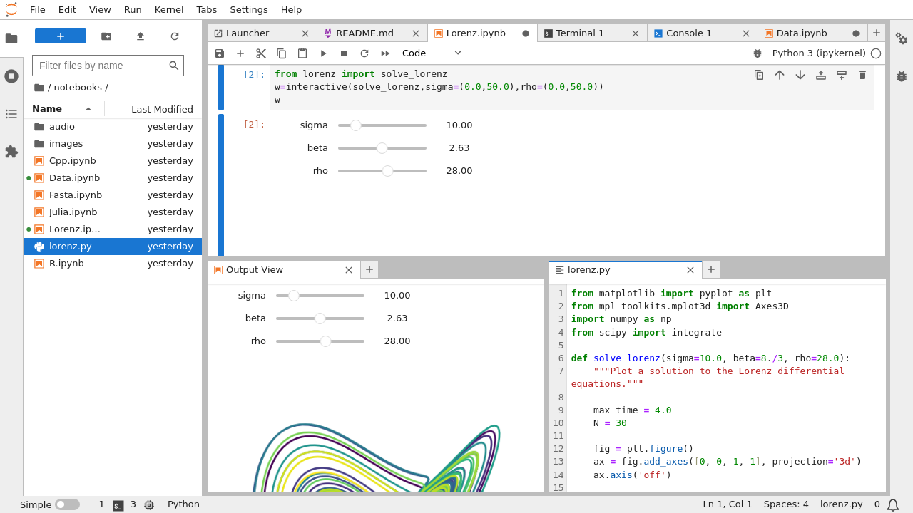
• full-fledged IDE, similar to e.g. Rstudio.
• Tab views, Code consoles, Show output in a separate tab, Live rendering of edits

conda install –c conda-forge jupyterlab

lets you build an online book using a collection of Jupyter Notebooks and Markdown files

• Interactivity
• Citations
• Build and host it online with GitHub/GitHub Pages...
• or locally on your own laptop

For the tutorial:

---

use jupyter notebook or jupyter lab

Questions?