
| Description | Hands On Lab Exercises for RNASeq assembly |
|---|---|
| Related-course materials | Linux for Dummies |
| Related-course materials | RNAseq |
| Authors | Julie Orjuela-Bouniol (julie.orjuela@ird.fr) - i-Trop platform (UMR BOREA / DIADE / IPME - IRD) |
| Creation Date | 02/08/2019 |
| Last Modified Date | 21/09/2019 |
| Modified by | Christine Tranchant (christine.tranchant@ird.fr) |
Summary
- Preambule : 0. Going to the i-Trop cluster -
ssh,srun,scp - Practice 1:# 1. Check Reads Quality
- Practice 2:# 2. Performing a de novo RNA-Seq assembly with
trinity - Practice 3:# 3. Assessing transcriptome assembly quality
- Practice 4:# 4. Differential Expression Analysis (DE)
- License
0. Going to the i-Trop cluster - ssh,srun,scp
Dataset used in this practical comes from
- ref : https://www.ncbi.nlm.nih.gov/pmc/articles/PMC3488244/
- data : NCBI SRA database under accession number SRS307298 S. cerevisiae
- Genome size of S. cerivisiae : 12M (12.157.105) (https://www.yeastgenome.org/strain/S288C#genome_sequence)
In this session, we will analyze RNA-seq data from one sample of S. cerevisiae (NCBI SRA SRS307298). It is from two different origin (CENPK and Batch), with three biological replications for each origin (rep1, rep2 and rep3).
Connection to the i-Trop Cluster through ssh mode
We will work on the i-Trop Cluster with a “supermem” node using SLURM scheduler.
ssh formationX@bioinfo-master.ird.frOpening an interactive bash session on the node25 (supermem partition) - srun -p partition --pty bash -i
Read this survival document containig basic commands to SLURM (https://southgreenplatform.github.io/trainings/slurm/)
srun -p supermem --mem 50G --time 20:00:00 --cpus-per-task 2 --pty bash -iPrepare input files
- Create your subdirectory in the scratch file system /scratch. In the following, please replace X with your own user ID number in formationX.
cd /scratch
mkdir formationX
cd formationX- Copy the exercise files from the shared location to your scratch directory (it is essential that all calculations take place here)
scp -r nas:/data2/formation/TP-trinity/SRA_SRS307298/RAWDATA/ /scratch/formationX/- When the files transfer is finished, verify by listing the content of the current directory and the subdirectory RAWDATA with the
command
ls -al. You should see 12 gzipped read files in a listing, thesamples.txtfile and therun_trinity.shbash script.
[orjuela@node25 RAWDATA]$ more samples.txt
CENPK	CENPK_rep1	PATH/SRR453569_1.fastq.gz	PATH/SRR453569_2.fastq.gz
CENPK	CENPK_rep2	PATH/SRR453570_1.fastq.gz	PATH/SRR453570_2.fastq.gz
CENPK	CENPK_rep3	PATH/SRR453571_1.fastq.gz	PATH/SRR453571_2.fastq.gz
Batch	Batch_rep1	PATH/SRR453566_1.fastq.gz	PATH/SRR453566_2.fastq.gz
Batch	Batch_rep2	PATH/SRR453567_1.fastq.gz	PATH/SRR453567_2.fastq.gz
Batch	Batch_rep3	PATH/SRR453568_1.fastq.gz	PATH/SRR453568_2.fastq.gz
1. Check Reads Quality
FastQC perform some simple quality control checks to ensure that the raw data looks good and there are no problems or biases in data which may affect how user can usefully use it. http://www.bioinformatics.babraham.ac.uk/projects/fastqc/
# make a fastqc repertoty
cd ../
mkdir FASTQC; cd FASTQC

#charge modules
module load bioinfo/FastQC/0.10.1

# run fastqc in the whole of samples
fastqc -t 2 /scratch/formationX/RAWDATA/*.gz -o /scratch/formationX/FASTQC/
Multiqc is a modular tool to aggregate results from bioinformatics analyses across many samples into a single report. Use this tool to visualise results of quality. https://multiqc.info/
#charge modules
module load bioinfo/multiqc/1.7

#launch Multiqc to create a report in html containing the whole of informations generated by FastQC
multiqc .

#transfer results to your cluster home
scp -r multiqc* nas:/home/formationX/

# transfert results to your local machine by scp or filezilla
scp -r formationX@bioinfo-nas.ird.fr:/home/formationX/multiqc* ./

# open in your favorite web navigator
firefox multiqc_report.html .
In this practice, reads quality is ok. You need to observe sequences and check biases. To remove adaptors and primers you can use Trimmomatic. Use PRINSEQ2 to detect Poly A/T tails and low complexity reads. Remove contaminations with SortMeRNA, riboPicker or DeconSeq.
2. Performing a de novo RNA-Seq assembly with trinity
2.1 Running Trinity with trimmomatic and reads normalisation
Preparing assembly sample file and check parameters of trinity assembler
Observe run_trinity.sh script and adapt to your formation number. This script is not sending in sbatch mode because it could be take time in this training. If you need launch it in a slurm cluster you can use this version containing SBATCH commands run_trinity.slurm or adapt it to SGE.
[orjuela@node25 RAWDATA]$ more run_trinity.sh

# loading modules
module load bioinfo/samtools/1.9
module load bioinfo/trinityrnaseq/2.8.5
module load bioinfo/Trimmomatic/0.33

# changing PATH to current directory in samples file
sed -i 's|PATH|'$PWD'|ig' samples.txt

# Running trinity assembly
# Trinity --seqType fq --max_memory 50G --CPU 2 --samples_file samples.txt --output ../TRINITY_OUT

# Running Trinity with trimmomatic and normalisation
Trinity --seqType fq --max_memory 50G --CPU 2 --trimmomatic --quality_trimming_params 'ILLUMINACLIP:/usr/local/Trimmomatic-0.33/adapters/TruSeq2-PE.fa:2:30:10 ILLUMINACLIP:/scratch/formationX/RAWDATA/adapt-125pbLib.txt:2:30:10 SLIDINGWINDOW:5:20 LEADING:5 TRAILING:5 MINLEN:25 HEADCROP:10' --normalize_by_read_set --samples_file samples.txt --output ../TRINITY_OUT
Running assembly :
bash run_trinity.sh > ../trinity.log & All screen output (info messages and error messages, if any) will be saved in the file
../trinity.log. The script will start executing in the background (the & at the end), so
that the terminal will return to the prompt right after you hit “Enter”.
You can use jobs to monitor jobs but if you logout the program does not keep running.
While running you can examine steps tail -f ../trinity.log.
After trimmomatic and reads normalisation, Three stages are done by Trinity
- Jellyfish: Extracts and counts K-mers (K=25) from reads
- Inchworm: Assembles initial contigs by “greedily” extending sequences with most abundant K-mers
- Chrysalis: Clusters overlapping Inchworm contigs, builds de Bruijn graphs for each cluster, partitions reads between clusters
- Butterfly: resolves alternatively spliced and paralogous transcripts independently for each cluster (in parallel)
Ending up assembly and downloading assembly results
-
WARNING !: This job is expected to run 12 hours. Kill your job using `fg` and `ctl+c`
 jobs = shows jobs running
 fg = foreground
 bf = background
 ctrl+z = send job to background
ctrl+c = kill job in ground- Recover assembly results (only Trinity.fasta) generated by trinity from the shared location to your scratch directory :
scp -r  nas:/data2/formation/TP-trinity/TRINITY_OUT/TRINITY_OUT/Trinity.fasta /scratch/formationX/

cd /scratch/formationX/TRINITY_OUT- Upon successful completion of Trinity, the assembled transcriptome is written to the FASTA file called
Trinity.fastalocated in the output directory/scratch/formationX/TRINITY_OUT.
3. Assessing transcriptome assembly quality
3.1 Getting basic Assembly metrics with the trinity script TrinityStats.pl
Running trinity script
Trinity.fasta contains transcripts to be evaluated, annotated, and used in downstream analysis of expression. In this exercise, we only concentrate on basis statistics of the assembled transcriptome, which can be obtained using a Trinity utility script TrinityStats.pl.
#declare the path_to_trinity variable
path_to_trinity=/usr/local/trinityrnaseq-2.8.5/
#check path
echo $path_to_trinity
#launch assembly metrics script
$path_to_trinity/util/TrinityStats.pl /scratch/formationX/TRINITY_OUT/Trinity.fasta > trinityStats.log
Parsing the results generated by the script
The output file generated (trinityStats.log) will contain basic information about contig length distributions, based on all transcripts and only on the longest isoform per gene.
Besides average and median contig lengths, also given are quantities N10 through N50. Nx is the smallest contig length such that (x/100)% of all assembled bases are in contigs longer than Nx. Specifically, N50 is the contig length such that half of all assembly sequence is contained in contigs longer than that. In whole genome assembly, N50 is often used as a measure (one of many) of assembly quality, since the longer the contigs, the better the assembly. In the case of transcriptome, contig lengths should be correct, which does not imply “large”. If it falls in the right ballpark (about 1000-1,500), N50 can still be used as a check on overall “sanity” of the transcriptome assembly.
[orjuela@node25 orjuela]$ more trinityStats.log

################################
## Counts of transcripts, etc.
################################
Total trinity 'genes':	7600
Total trinity transcripts:	8616
Percent GC: 39.37

########################################
Stats based on ALL transcript contigs:
########################################

	Contig N10: 11180
	Contig N20: 8394
	Contig N30: 6793
	Contig N40: 5553
	Contig N50: 4736

	Median contig length: 506
	Average contig: 1909.88
	Total assembled bases: 16455500


#####################################################
## Stats based on ONLY LONGEST ISOFORM per 'GENE':
#####################################################

	Contig N10: 9989
	Contig N20: 7558
	Contig N30: 6192
	Contig N40: 5131
	Contig N50: 4194

	Median contig length: 423
	Average contig: 1625.41
	Total assembled bases: 12353135
3.2 Reads mapping back rate and abundance estimation using the trinity script align_and_estimate_abundance.pl
Read congruency is an important measure in determining assembly accuracy. Clusters of read pairs that align incorrectly are strong indicators of mis-assembly. A typical “good” assembly has ~80% reads mapping to the assembly and ~80% are properly paired.
Several tools can be used to calculate reads mapping back rate over Trinity.fasta assembly : bwa, bowtie2 (mapping), kallisto, salmon (pseudo mapping). Quantify read counts for each gene/isoform can be calculate. Mapping and quantification can be obtained by using the –est_method argument into the align_and_estimate_abundance.pl script.
We will performing this analyses step successively with the align_and_estimate_abundance.pl script :
- Pseudomapping methods (kallisto or salmon) are faster than mapping based. So firstly we will use salmon to pseudoalign reads from sample to the reference and quantify abondance.
- Then, we will use bowtie2 and RSEM to align and quantify read counts for each gene/isoform.
Preparing data and environment for our following analysis
#create a directory dans /scratch/formationX/
mkdir ALIGN_AND_ABUNDANCE
cd ALIGN_AND_ABUNDANCE

# Loading modules
module load system/perl/5.24.0
module load bioinfo/trinityrnaseq/2.8.5
module load bioinfo/bowtie2/2.2.9
module load bioinfo/express/1.5.1
module load bioinfo/kallisto/0.43.1
module load bioinfo/RSEM/1.0
module load bioinfo/salmon/0.10.2
module load bioinfo/samtools/1.7

# modifying samples file path because quality-trimmed your reads using the --trimmomatic parameter in Trinity
cp /scratch/formationX/RAWDATA/samples.txt .
sed -i 's|RAWDATA|TRINITY_OUT|ig' samples.txt
sed -i 's|.fastq.gz|.fastq.gz.P.qtrim.gz|ig' samples.txt

# define variables
path_to_trinity=/usr/local/trinityrnaseq-2.8.5/
fasta=/scratch/formationX/TRINITY_OUT/Trinity.fasta
samplesfile=/scratch/formationX/ALIGN_AND_ABUNDANCE/samples.txt #modified samples file
Launch Salmon
# create a salmon_outdir and go on
mkdir salmon_outdir; cd salmon_outdir

# salmon
perl $path_to_trinity/util/align_and_estimate_abundance.pl \
--transcripts $fasta \
--seqType fq \
--samples_file $samplesfile \
--est_method salmon \
--trinity_mode \
--prep_reference > salmon_align_and_estimate_abundance.log 2>&1 &
Check reads percentage mapped to Trinity.fasta reference by sample for salmon and bowtie-rsem est method.
#salmon results
[orjuela@node25 salmon_outdir]$ grep 'Mapping rate =' */logs/salmon_quant.log
Batch_rep1/logs/salmon_quant.log:[2019-09-17 15:54:32.923] [jointLog] [info] Mapping rate = 96.3027%
Batch_rep2/logs/salmon_quant.log:[2019-09-17 15:55:09.922] [jointLog] [info] Mapping rate = 96.3992%
Batch_rep3/logs/salmon_quant.log:[2019-09-17 15:55:39.246] [jointLog] [info] Mapping rate = 96.7795%
CENPK_rep1/logs/salmon_quant.log:[2019-09-17 15:52:56.609] [jointLog] [info] Mapping rate = 94.4516%
CENPK_rep2/logs/salmon_quant.log:[2019-09-17 15:53:30.146] [jointLog] [info] Mapping rate = 95.0558%
CENPK_rep3/logs/salmon_quant.log:[2019-09-17 15:54:00.196] [jointLog] [info] Mapping rate = 95.0639%
OPTIONAL: Launch bowtie2-rsem
-
WARNING !: this job can take a lot ~1h30 by sample. This step will not run in this practice.
# create a bowtie2-rsem_outdir and go on
cd /scratch/formationX/ALIGN_AND_ABUNDANCE/
mkdir bowtie2-rsem_outdir; cd bowtie2-rsem_outdir

# runnign align_and_estimate_abundance in bowtie2-rsem mode
perl $path_to_trinity/util/align_and_estimate_abundance.pl \
--transcripts $fasta \
--seqType fq \
--samples_file $samplesfile \
--est_method RSEM --aln_method bowtie2 \
--trinity_mode \
--prep_reference \
--coordsort_bam > bowtie-rsem_align_and_estimate_abundance.log 2>&1 &
Here, we show you results with bowtie2-rsem OPTIONAL part
#bowtie-rsem results
[orjuela@node25 bowtie2-rsem_outdir]$ grep -B 6 "overall alignment rate" bowtie-rsem_align_and_estimate_abundance.log
CMD: set -o pipefail && bowtie2 --no-mixed --no-discordant --gbar 1000 --end-to-end -k 200  -q -X 800 -x /scratch/orjuela/TRINITY_OUT/Trinity.fasta.bowtie2 -1 /scratch/orjuela/TRINITY_OUT/SRR453569_1.fastq.gz.P.qtrim.gz -2 /scratch/orjuela/TRINITY_OUT/SRR453569_2.fastq.gz.P.qtrim.gz -p 4 | samtools view -@ 4 -F 4 -S -b | samtools sort -@ 4 -n -o bowtie2.bam
3666948 reads; of these:
  3666948 (100.00%) were paired; of these:
    497221 (13.56%) aligned concordantly 0 times
    2058938 (56.15%) aligned concordantly exactly 1 time
    1110789 (30.29%) aligned concordantly >1 times
86.44% overall alignment rate
--
 ...
3.3. Expression matrix construction
Combine read count from all samples into a matrix, and normalize the read count using the TMM method. This command will take in RSEM output files from each sample, and combine them into a single matrix file.
# go to salmon results repertory
cd /scratch/formationX/ALIGN_AND_ABUNDANCE/salmon_outdir

#load modules
module load bioinfo/R/3.3.3
module load system/perl/5.24.0

#declare bash variables
path_to_trinity=/usr/local/trinityrnaseq-2.8.5/

# calculate expression matrix (if salmon use quant.sf files, if kallisto use abundance.tsv files)
$path_to_trinity/util/abundance_estimates_to_matrix.pl \
--est_method salmon \
--out_prefix Trinity_trans \
--name_sample_by_basedir \
--gene_trans_map none \
CENPK_rep1/quant.sf \
CENPK_rep2/quant.sf \
CENPK_rep3/quant.sf \
Batch_rep1/quant.sf \
Batch_rep2/quant.sf \
Batch_rep3/quant.sf
You have to obtain two matrices:
The firts one containing the estimated counts ̀Trinity_trans.isoform.counts.matrix and the second one containing the TPM expression values that are cross-sample normalized using the TMM method Trinity_trans.TMM.EXPR.matrix.
TMM normalization assumes that most transcripts are not differentially expressed, and linearly scales the expression values of samples to better enforce this property.
In both files, each column represents a sample, and each row represents a gene, the values are either the raw read counts or normalized FPKM values. The “counts” file will be used for differentially expressed gene identification, and the “fpkm” file will be used for clustering analysis. By default, the fpkm file is normalized with TMM method.
[orjuela@node25 salmon_outdir]$ ll Trinity_trans.*
total 1,4M
-rw-r--r-- 1 orjuela borea-equipe7 539K 29 août  16:41 Trinity_trans.isoform.TMM.EXPR.matrix
-rw-r--r-- 1 orjuela borea-equipe7 386K 29 août  16:41 Trinity_trans.isoform.counts.matrix
-rw-r--r-- 1 orjuela borea-equipe7 474K 29 août  16:41 Trinity_trans.isoform.TPM.not_cross_norm
-rw-r--r-- 1 orjuela borea-equipe7  355 29 août  16:41 Trinity_trans.isoform.TPM.not_cross_norm.TMM_info.txt
-rw-r--r-- 1 orjuela borea-equipe7  542 29 août  16:41 Trinity_trans.isoform.TPM.not_cross_norm.runTMM.R

[orjuela@node25 salmon_outdir]$ head *.matrix
==> Trinity_trans.isoform.counts.matrix <==
	CENPK_rep1	CENPK_rep2	CENPK_rep3	Batch_rep1	Batch_rep2	Batch_rep3
TRINITY_DN3130_c0_g1_i1	0.000000	4.000000	0.000000	0.000000	0.000000	0.000000
TRINITY_DN986_c0_g1_i4	190.000000	210.677452	319.000000	353.571187	420.080043	292.000000
TRINITY_DN4062_c0_g2_i1	0.000000	13.000000	0.000000	0.000000	0.000000	0.000000
TRINITY_DN4840_c0_g1_i1	0.000000	10.000000	0.000000	0.000000	0.000000	0.000000
TRINITY_DN1624_c0_g1_i1	0.000000	5.000000	0.000000	0.000000	0.000000	0.000000
TRINITY_DN3492_c0_g1_i1	0.000000	5.000000	0.000000	0.000000	0.000000	0.000000
TRINITY_DN1386_c0_g1_i1	671.000000	724.000000	997.000000	1325.000000	1726.000000	1229.000000
TRINITY_DN6688_c0_g1_i1	0.000000	5.000000	0.000000	0.000000	0.000000	0.000000
TRINITY_DN1126_c0_g2_i1	29.000000	42.000000	51.000000	14.000000	7.000000	5.000000

==> Trinity_trans.isoform.TMM.EXPR.matrix <==
	CENPK_rep1	CENPK_rep2	CENPK_rep3	Batch_rep1	Batch_rep2	Batch_rep3
TRINITY_DN3130_c0_g1_i1	0.000	32.382	0.000	0.000	0.000	0.000
TRINITY_DN986_c0_g1_i4	141.255	131.008	158.103	195.483	180.432	173.943
TRINITY_DN4062_c0_g2_i1	0.000	20.291	0.000	0.000	0.000	0.000
TRINITY_DN4840_c0_g1_i1	0.000	23.121	0.000	0.000	0.000	0.000
TRINITY_DN1624_c0_g1_i1	0.000	22.187	0.000	0.000	0.000	0.000
TRINITY_DN3492_c0_g1_i1	0.000	30.511	0.000	0.000	0.000	0.000
TRINITY_DN1386_c0_g1_i1	96.472	86.724	94.337	140.804	141.542	140.796
TRINITY_DN6688_c0_g1_i1	0.000	23.740	0.000	0.000	0.000	0.000
TRINITY_DN1126_c0_g2_i1 9.819 11.863 11.412 3.511 1.357 1.351[orjuela@node25 salmon_outdir]$ more Trinity_trans.isoform.TPM.not_cross_norm.TMM_info.txt
group lib.size norm.factors eff.lib.size
CENPK_rep1 999995 1.14115425493455 1141148.54916327
CENPK_rep2 999993 0.905154412329735 905148.076248848
CENPK_rep3 1000003 1.0939694255262 1093972.70743448
Batch_rep1 999992 0.989872299588587 989864.38061019
Batch_rep2 999990 0.950965458077021 950955.94842244
Batch_rep3 1000015 0.940121262909323 940135.3647282663.4 Compute N50 based on the top-most highly expressed transcripts (Ex50)
$path_to_trinity/util/misc/contig_ExN50_statistic.pl Trinity_trans.isoform.TMM.EXPR.matrix /scratch/formationX/TRINITY_OUT/Trinity.fasta > ExN50.stats

#Plotting ExN50
$path_to_trinity/util/misc/plot_ExN50_statistic.Rscript ExN50.stats

#If you want to know, how many transcripts correspond to the Ex 90 peak, you could:
cat Trinity_trans.isoform.TMM.EXPR.matrix.E-inputs |  egrep -v ^\# | awk '$1 <= 90' | wc -l
1761

# or 50
cat Trinity_trans.isoform.TMM.EXPR.matrix.E-inputs |  egrep -v ^\# | awk '$1 <= 50' | wc -l
163
TRANSFERT: Observe plots. Remember, you have to transfert *.pdf files to your home before of transfering into your local machine.
#transfering plots
cp *.pdf /home/formationX/
# from your local machine
scp formationX@bioinfo-nas.ird.fr:*.pdf .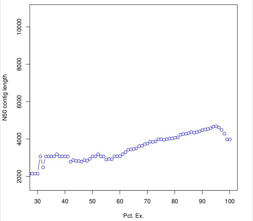
3.5 Quantifying completness using BUSCO
Assessing gene space is a core aspect of knowing whether or not you have a good assembly.
Benchmarking Universal Single-Copy Orthologs (BUSCO) sets are collections of orthologous groups with near-universally-distributed single-copy genes in each species, selected from OrthoDB root-level orthology delineations across arthropods, vertebrates, metazoans, fungi, and eukaryotes. BUSCO groups were selected from each major radiation of the species phylogeny requiring genes to be present as single-copy orthologs in at least 90% of the species; in others they may be lost or duplicated, and to ensure broad phyletic distribution they cannot all be missing from one sub-clade. The species that define each major radiation were selected to include the majority of OrthoDB species, excluding only those with unusually high numbers of missing or duplicated orthologs, while retaining representation from all major sub-clades. Their widespread presence means that any BUSCO can therefore be expected to be found as a single-copy ortholog in any newly-sequenced genome from the appropriate phylogenetic clade.
Running Busco on Trinity.fasta assembly
#make a BUSCO directory
cd /scratch/formationX/
mkdir BUSCO; cd BUSCO
# download the eukaryota database from https://busco.ezlab.org/
# There is a lot of other databases usable for this dataset (ex: Fungi gene set or Saccaromyceta gene set, with more genes to retrieve, so longer to run)

wget https://busco.ezlab.org/datasets/eukaryota_odb9.tar.gz
# uncompress repertory
tar zxvf eukaryota_odb9.tar.gz

# define variables
busco=/usr/local/BUSCO-3.0.2/scripts/run_BUSCO.py
path_to_trinity=/usr/local/trinityrnaseq-2.8.5/
fasta=/scratch/formationX/TRINITY_OUT/Trinity.fasta
LINEAGE=/scratch/formationX/BUSCO/eukaryota_odb9

# run busco
/usr/local/python-3.6.5/bin/python $busco -i $fasta -l $LINEAGE -m transcriptome  -c 2 -o trinity_busco > busco.log &

# check busco running using
jobs
# or
tail -f busco.log
Displaying the short summary table generated by BUSCO
[orjuela@node25 run_trinity_busco]$ more run_trinity_busco/short_summary_trinity_busco.txt
# BUSCO version is: 3.0.2
# The lineage dataset is: eukaryota_odb9 (Creation date: 2016-11-02, number of species: 100, number of BUSCOs: 303)
# To reproduce this run: python /usr/local/BUSCO-3.0.2/scripts/run_BUSCO.py -i /scratch/formation1/TRINITY_OUT/Trinity.fasta -o trinity_busco_euk -l /scratch/formation1/BUSCO/eukaryota_odb9/ -m transcriptome -c 2

#
# Summarized benchmarking in BUSCO notation for file /scratch/orjuela/TRINITY_OUT/Trinity.fasta
# BUSCO was run in mode: transcriptome

	C:93.4%[S:74.6%,D:18.8%],F:0.0%,M:6.6%,n:303

	283	Complete BUSCOs (C)
	226	Complete and single-copy BUSCOs (S)
	57	Complete and duplicated BUSCOs (D)
	0	Fragmented BUSCOs (F)
	20	Missing BUSCOs (M)
	303	Total BUSCO groups searched
3.6 BLASTX comparison to known protein sequences database
Performing a blastx againt the swissprot database (the manually annotated and reviewed section of the UniProt Knowledgebase)
-
WARNING !: This step will not run in this practice because it will be inclued in annotation script !! But we give you commands lines to lauch with your data.
#load modules
module load bioinfo/blast/2.4.0+

#define variables
path_to_blast=/usr/local/ncbi-blast-2.4.0+/bin/
path_to_trinity=/usr/local/trinityrnaseq-2.8.5/

# create BLASTX repertory
mkdir /scratch/formationX/BLASTX
cd /scratch/formationX/BLASTX

# First, we downloaded and indexed the database from ftp://ftp.ebi.ac.uk/pub/databases/uniprot/current_release/knowledgebase/complete/uniprot_sprot.fasta.gz,
# uniprotdatabase is available on cluster at  (with the correct index files)
uniprot=/data/projects/banks/Uniprot/uniprot_sprot.fasta

#Then, we ran BLASTX to get the top match hit:
$path_to_blast/blastx \
-db $uniprot \
-query $fasta \
-num_threads 2 \
-max_target_seqs 1 \
-outfmt 6 \
-evalue 1e-20 > SwissProt_1E20_Trinity_blastx.outfmt6 &

#if you want to test blastX practice, please recover results from `/data2/formation/TP-trinity/TRINITY_OUT/BLASTX/`

#Finally, we examined the percent of alignment coverage:
$path_to_trinity/util/misc/blast_outfmt6_group_segments.pl SwissProt_1E20_Trinity_blastx.outfmt6 $fasta $uniprot > SwissProt_1E20_Trinity_blastx.outfmt6.grouped

$path_to_trinity/util/misc/blast_outfmt6_group_segments.tophit_coverage.pl SwissProt_1E20_Trinity_blastx.outfmt6.grouped \
> SwissProt_1E20_Trinity_blastx.outfmt6.grouped.output
Analyzing blast results
[orjuela@node25 BLASTX]$ more SwissProt_1E20_Trinity_blastx.outfmt6.grouped.output
#hit_pct_cov_bin	count_in_bin	>bin_below
100	242	242
90	8	250
80	4	254
70	5	259
60	4	263
50	5	268
40	4	272
30	2	274
20	2	276
10	1	277
8616 transcripts from Trinity.fasta file were blasted against the swissprot database.
440 hits were reported in SwissProt_1E20_Trinity_blastx.outfmt6 file.
In SwissProt_1E20_Trinity_blastx.outfmt6.grouped.output file we can observed for example that 242 sequences were found with a 100% identity to an uniprot protein (count_in_bin). bin_below column represent a accumulative number of sequences.
4. Differential Expression Analysis (DE)
4.1 Examine your data and your experimental replicates before DE
Before differential expression analysis, examine your data to determine if there are any confounding issues. Trinity comes with a ‘PtR’ script that we use to simplify making various charts and plots based on a matrix input file. Run these three commands lines :
# go to salmon results repertory
cd /scratch/formationX/ALIGN_AND_ABUNDANCE/salmon_outdir

#create design file from samples.txt
cut -f1,2 ../samples.txt > design.txt

[orjuela@node25 salmon_outdir]$ more design.txt
CENPK	CENPK_rep1
CENPK	CENPK_rep2
CENPK	CENPK_rep3
Batch	Batch_rep1
Batch	Batch_rep2
Batch	Batch_rep3
Run PtR scripts
$path_to_trinity/Analysis/DifferentialExpression/PtR  --matrix Trinity_trans.isoform.counts.matrix --samples design.txt --log2 --min_rowSums 10 --compare_replicates

$path_to_trinity/Analysis/DifferentialExpression/PtR  --matrix Trinity_trans.isoform.counts.matrix --samples design.txt --log2 --min_rowSums 10 --CPM --sample_cor_matrix

$path_to_trinity/Analysis/DifferentialExpression/PtR  --matrix Trinity_trans.isoform.counts.matrix --samples design.txt --log2 --min_rowSums 10  --CPM --center_rows --prin_comp
TRANSFERT : Observe plots. Remember, you have to transfert *.pdf files to your home before of transfering into your local machine.
#transfering plots
cp *.pdf /home/formationX/
# from your local machine
scp formationX@bioinfo-nas.ird.fr:*.pdf .
Results can be found here
4.2 Identify differentially expressed genes between the two tissues.
The tool run_DE_analysis.pl is a PERL script that use Bioconductor package edgeR.
#run DE analysis
$path_to_trinity/Analysis/DifferentialExpression/run_DE_analysis.pl \
--matrix Trinity_trans.isoform.counts.matrix \
--method edgeR \
--samples_file design.txt \
--output edgeR_results
The output files are in the directory edgeR_results. Observe file Trinity_trans.isoform.counts.matrix.Batch_vs_CENPK.edgeR.DE_results. It provides several values for each gene:
1) FDR to indicate whether a gene is differentially expressed or not
2) logFC is the log2 transformed fold change between the two tissues
3) logCPM is the log2 transformed normalized read count of average of the samples.
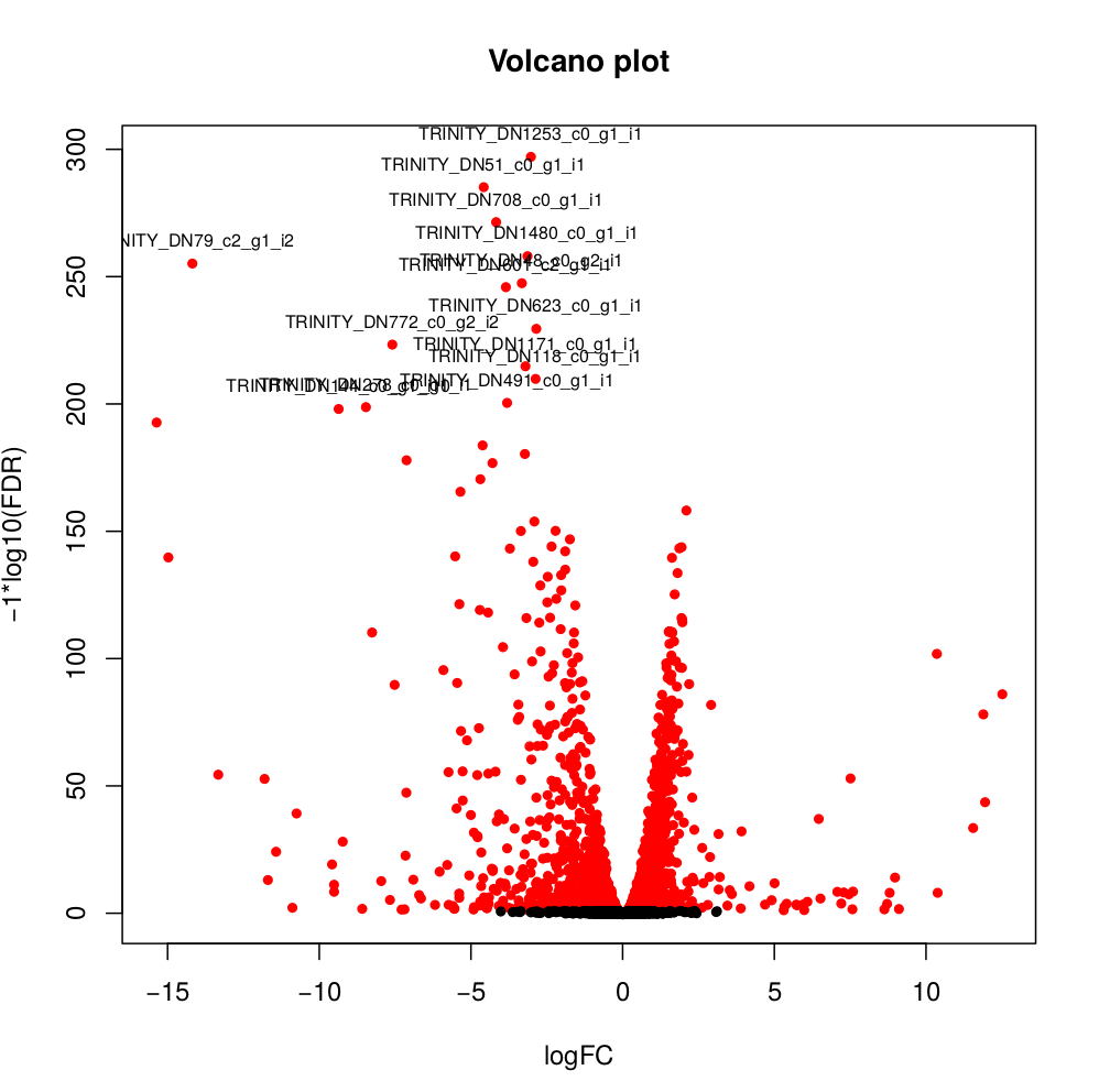
Usually you have to filter this list of genes/isoforms to FDR <0.05 or below. To be more conservative, you could also use more stringent FDR cutoff (e.g. <0.001), and only keep genes with high logFC (e.g. <-2 and >2) and/or high logCPM (e.g. >1). In the edgeR_results directory there is also a “volcano plot” to visualize the distribution of the DE genes.
[orjuela@node25 salmon_outdir]$ head edgeR_results/Trinity_trans.isoform.counts.matrix.Batch_vs_CENPK.edgeR.DE_results
sampleA	sampleB	logFC	logCPM	PValue	FDR
TRINITY_DN332_c0_g1_i10	Batch	CENPK	-10.359903780639	8.33512668205486	0	0
TRINITY_DN730_c0_g2_i1	Batch	CENPK	-6.4740873961699	8.70152404919916	0	0
TRINITY_DN741_c0_g1_i1	Batch	CENPK	-6.31231314146213	10.2830859720565	0	0
TRINITY_DN287_c1_g1_i1	Batch	CENPK	-6.26650019458591	8.47203996977476	0	0
TRINITY_DN65_c0_g1_i3	Batch	CENPK	-4.13189957112457	10.730475730689	0	0
TRINITY_DN1298_c0_g1_i1	Batch	CENPK	-3.19109633696326	8.91247526735535	0	0
TRINITY_DN1253_c0_g1_i1	Batch	CENPK	-3.03997649547823	8.99502681145441	6.47317750883953e-301	3.75444295512693e-298
TRINITY_DN51_c0_g1_i1	Batch	CENPK	-4.59451625218422	10.4521118447878	5.94332889429699e-289	3.01623941385572e-286
TRINITY_DN708_c0_g1_i1	Batch	CENPK	-4.1838974791094	7.70916912374135	3.84699757684993e-275	1.73542335133453e-272
#transfering plots
cd edgeR_result
cp *.pdf /home/formationX/
# from your local machine
scp formationX@bioinfo-nas.ird.fr:*.pdf .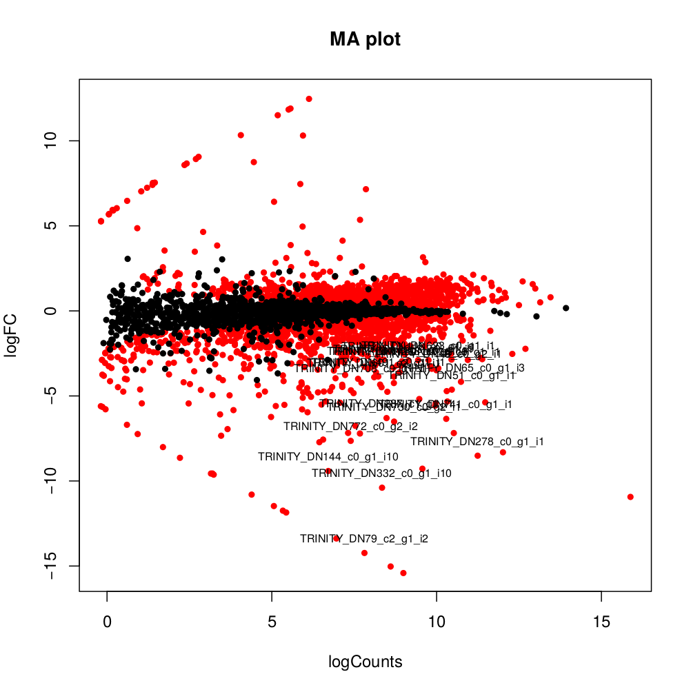
4.3 Clustering analysis
Hierarchical clustering and k-means clustering for samples and genes can be done using trinity scripts.
The clustering will be performed only on differentially expressed genes, with FDR and logFC cutoff defined by -P and -C parameters.
In this example, we set K=4 for k-means analysis. The genes will be separated into 4 groups based on expression pattern.
There are two prefiltered files produced: *DE_results.P1e-3_C2.Batch-UP.subset and *DE_results.P1e3_C2.CENPK-UP.subset, with differentially expressed genes (FDR cutoff 0.001, logFC cutoff 2 and -2).
#go to edgeR_results
cd edgeR_results
# running analyze_diff_expr
$path_to_trinity/Analysis/DifferentialExpression/analyze_diff_expr.pl \
--matrix ../Trinity_trans.isoform.TMM.EXPR.matrix --samples ../design.txt -P 1e-3 -C 2 \
--output cluster_results
# running define_clusters_by_cutting_tree
$path_to_trinity/Analysis/DifferentialExpression/define_clusters_by_cutting_tree.pl \
-K 4 -R cluster_results.matrix.RData
#transfering plots
cp *.pdf /home/formationX/
# from your local machine
scp formationX@bioinfo-nas.ird.fr:*.pdf .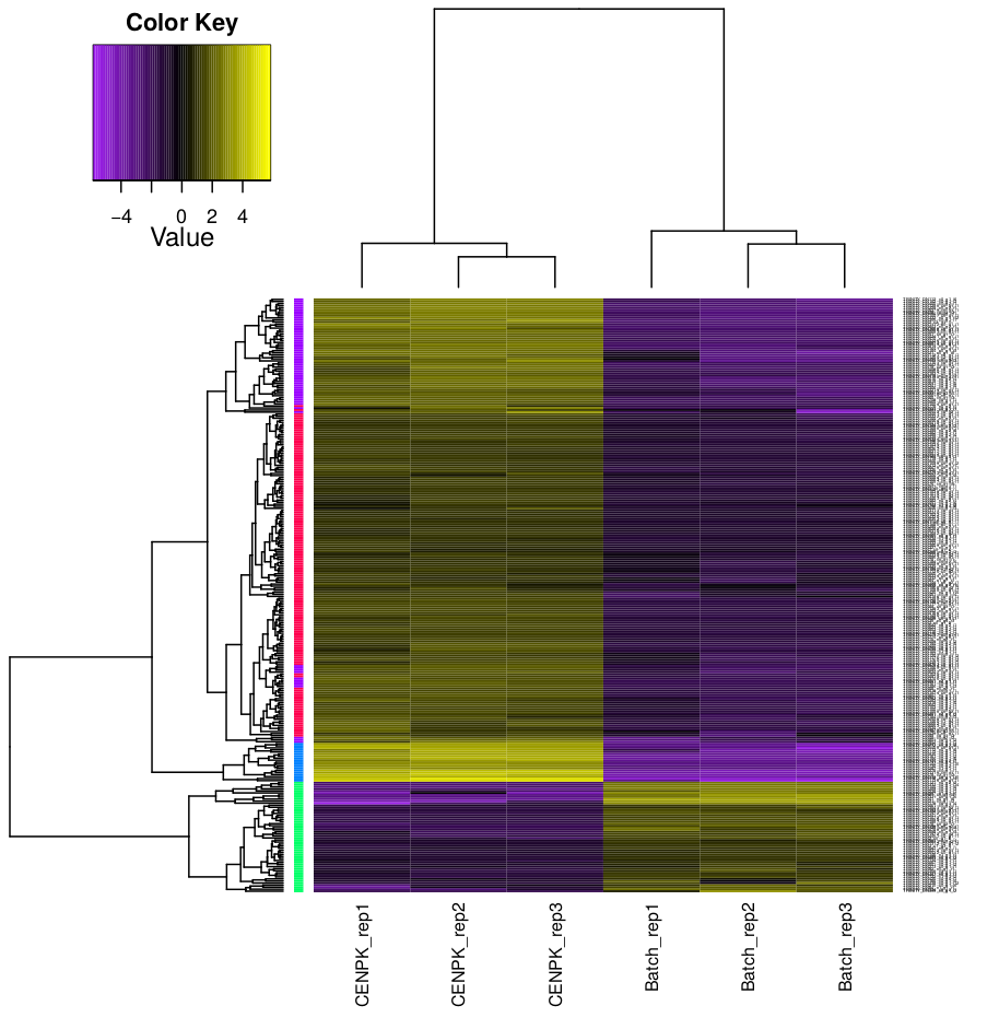
Before finish …
Go to here to recover the scripts used in this training.
License
