
| Description | Hands On Lab Exercises for RNASeq |
|---|---|
| Related-course materials | Transcriptomique |
| Related-course materials | Trinity and Trinotate |
| Related-course materials | Linux for Dummies |
| Authors | Julie Orjuela (julie.orjuela_AT_irf.fr), Christine Tranchant (christine.tranchant_AT_ird.fr) |
| Creation Date | 15/03/2018 |
| Last Modified Date | 03/10/2019 |
Summary
- Preambule 0: Connection into cluster -
ssh,srun,scp - Practice 1: Check Reads Quality
- Practice 2: Pseudo-mapping against transcriptome reference + counting with Kallisto
- Practice 3: Mapping against annotated genome reference with Hisat2 + counting with Stringtie
- Practice 4: Visualization of mapped reads against genes using IGV
- Practice 5: Differential Expression Analysis (DE) using scripts associated with Trinity software
- Practice 6: Differential expression analysis with EdgeR and DESeq2 using PIVOT
- Links
- License
Practice 0. Going to the cluster - ssh,srun,scp
Dataset used in this practical comes from
- ref : https://www.ncbi.nlm.nih.gov/pmc/articles/PMC3488244/
- data : NCBI SRA database under accession number SRS307298 S. cerevisiae.
- Genome size of S. cerevisiae : 12M (12.157.105) (https://www.yeastgenome.org/strain/S288C#genome_sequence)
In this session, we will analyze RNA-seq data from one sample of S. cerevisiae (NCBI SRA SRS307298). It is from two different origin (CENPK and Batch), with three biological replications for each origin (rep1, rep2 and rep3).
Connection into cluster through ssh mode
We will work on the cluster of the Joseph KI-ZERBI University (UJKZ) using SLURM scheduler.
ssh formationX@YOUR_IP_ADRESSOpening an interactive bash session on a node srun -p partition --pty bash -i
Read this survival document containig basic commands to SLURM (https://southgreenplatform.github.io/trainings/slurm/)
srun -p PARTITIONNAME --time 08:00:00 --cpus-per-task 2 --pty bash -iPrepare input files
- Create your subdirectory in the scratch file system /scratch. In the following, please replace X with your own user ID number in formationX.
# declare PATHTODATA variable : in this TP data are in /scratch/SRA_SRS307298
PATHTODATA="/PATH/TO/DATA/"

# create scratch repertory
cd /scratch
mkdir formationX
cd formationX
Link files from the shared location from scratch directory (it is essential that all calculations take place here). But keep in mind that your data can be located in your /home or on a NAS for example.
ln -s $PATHTODATA/SRA_SRS307298/RAWDATA/ /scratch/formationX/When the files transfer is finished, verify by listing the content of the current directory and the subdirectory RAWDATA with the command ls -al. You should see 12 gzipped read files in a listing, a samples.txt file and a adapt-125pbLib.txt file.
[orjuela@node25 RAWDATA]$ more samples.txt
CENPK	CENPK_rep1	PATH/SRR453569_1.fastq.gz	PATH/SRR453569_2.fastq.gz
CENPK	CENPK_rep2	PATH/SRR453570_1.fastq.gz	PATH/SRR453570_2.fastq.gz
CENPK	CENPK_rep3	PATH/SRR453571_1.fastq.gz	PATH/SRR453571_2.fastq.gz
Batch	Batch_rep1	PATH/SRR453566_1.fastq.gz	PATH/SRR453566_2.fastq.gz
Batch	Batch_rep2	PATH/SRR453567_1.fastq.gz	PATH/SRR453567_2.fastq.gz
Batch	Batch_rep3	PATH/SRR453568_1.fastq.gz	PATH/SRR453568_2.fastq.gz
Practice 1. Check Reads Quality
FastQC perform some simple quality control checks to ensure that the raw data looks good and there are no problems or biases in data which may affect how user can usefully use it. http://www.bioinformatics.babraham.ac.uk/projects/fastqc/
# make a fastqc repertoty
cd /scratch/formationX
mkdir FASTQC
cd FASTQC

# charge modules
module load fastqc/0.11.7/

# run fastqc in the whole of samples (it will take 10min)
fastqc -t 1 /scratch/formationX/RAWDATA/*.gz -o /scratch/formationX/FASTQC/
Multiqc is a modular tool to aggregate results from bioinformatics analyses across many samples into a single report. Use this tool to visualise results of quality. https://multiqc.info/
#charge modules
module load MultiQC/1.7

#launch Multiqc to create a report in html containing the whole of informations generated by FastQC
multiqc .

#transfer results to your cluster home
scp -r multiqc* master:/home/formationX/

# transfert results FROM your local machine by scp or filezilla
scp -r formationX@:YOUR_IP_ADRESS /home/formationX/multiqc* ./

# open in your favorite web navigator
firefox multiqc_report.html .
In this practice, reads quality is ok. You need to observe sequences and check biases. To remove adaptors and primers you can use Trimmomatic. Use PRINSEQ2 to detect Poly A/T tails and low complexity reads. Remove contaminations with SortMeRNA, riboPicker or DeconSeq.
1.1 Cleanning reads with trimmomatic
# make a fastqc repertoty
cd /scratch/formationX
mkdir TRIMMOMATIC
cd TRIMMOMATIC

# loading modules
module load Trimmomatic/0.38

# Copy samples file and changing PATH to current directory in samples file.
cp ../RAWDATA/samples.txt .
sed -i 's|PATH|'$PWD'|ig' samples.txt
Running trimmomatic for each sample
In this example, reads of SRR453566 sample are trimmed. (_U untrimmed _P paired)
-
ILUMINACLIP is used to find and remove Illumina adapters.
-
SLIDINGWINDOW performs a sliding window trimming, cutting once the average quality within the window falls below a threshold. By considering multiple bases, a single poor quality base will not cause the removal of high quality data later in the read.
-
LEADING removes low quality bases from the beginning. As long as a base has a value below this threshold the base is removed and the next base will be investigated.
-
TRAILING specifies the minimum quality required to keep a base
-
MINLEN removes reads that fall below the specified minimal length
java -jar /usr/local/Trimmomatic-0.38/trimmomatic-0.38.jar PE -phred33 /scratch/formationX/RAWDATA/SRR453567_1.fastq.gz /scratch/formationX/RAWDATA/SRR453567_2.fastq.gz SRR453567_1.P.fastq.gz SRR453567_1.U.fastq.gz SRR453567_2.P.fastq.gz SRR453567_2.U.fastq.gz ILLUMINACLIP:/scratch/formationX/RAWDATA/adapt-125pbLib.txt:2:30:10 SLIDINGWINDOW:4:5 LEADING:5 TRAILING:5 MINLEN:25In this example :
Input Read Pairs: 7615732 Both Surviving: 7504326 (98,54%) Forward Only Surviving: 71456 (0,94%) Reverse Only Surviving: 11202 (0,15%) Dropped: 28748 (0,38%)
TrimmomaticPE: Completed successfully
1.2 Check quality after trimming
Observe effet of trimming in your samples. Run fastqc in the whole of trimmed reads and observe it with MultiQC
Practice 2. Indexing references files
2.1 indexing a reference file
We will index references with kallisto index, samtools index to prepare references to follow analysis.
# load modules
module load R/3.5.0
module load samtools/1.8
module load perl/5.24.0
module load trinity/2.8.5
#module load express/1.5.1
module load kallisto/0.44.0


# copy transcrits fasta reference file
cp -r $PATHTODATA/SRA_SRS307298/REF /scratch/formationX/

# go to REF repertoty
cd /scratch/formationX/REF

# index reference
kallisto index -i GCF_000146045.2_R64_genes.fai GCF_000146045.2_R64_genes.fasta
Practice 3. Mapping against transcriptome reference + counting with Kallisto
3.1 Kallisto
Now, we will perform a transcriptome-based mapping and estimates of transcript levels using Kallisto, and a differential analysis using EdgeR.
- Transfert references of transcriptome (cDNA) to be used as reference and index it, prepare a samples file and run kallisto for each sample
# declare bash variables
path_to_trinity=/usr/local/trinityrnaseq-Trinity-v2.8.5/
fasta=/scratch/formationX/REF/GCF_000146045.2_R64_genes.fasta
samplesfile=/scratch/SRA_SRS307298/KALLISTO/samples.txt

# make a KALLISTO repertory and go on
cd /scratch/formationX
mkdir KALLISTO
cd KALLISTO

# symbolic link to trimmed fastq
ln -s /scratch/SRA_SRS307298/TRIMMOMATIC/*.P.fastq.gz .

# Run the kallisto quant program by providing `GCF_000146045.2_R64_genes.fasta` as transcriptome reference and specifying correctly pairs of input fastq- `kallisto quant`- For every sample you have to run kallisto quant (example with SRR453568 sample) by using
kallisto quant -i GCF_000146045.2_R64_genes.fai -o SRR453568 <(zcat SRR453568_1.P.fastq.gz) <(zcat SRR453568_2_P.fastq.gz)command for example BUT we propose you use a trinity scriptalign_and_estimate_abundance.plto lauch the whole of samples in a command line.
# Create and modify samples file path
cp /scratch/formationX/RAWDATA/samples.txt .

# changing PATH to current directory in samples file
sed -i 's|PATH|'$PWD'|ig' samples.txt
sed -i 's|_1|_1.P|ig' samples.txt
sed -i 's|_2|_2.P|ig' samples.txt

# lauch kallisto using  `align_and_estimate_abundance.pl`
perl $path_to_trinity/util/align_and_estimate_abundance.pl \
--transcripts $fasta \
--seqType fq \
--samples_file $samplesfile \
--est_method kallisto \
--prep_reference > kallisto_align_and_estimate_abundance.log 2>&1- Visualize data abundance results
[orjuela@node25 KALLISTO]$ more CENPK_rep1/abundance.tsv
target_id	length	eff_length	est_counts	tpm
NC_001133.9:1807-2169	362	184.532	1	0.885838
NC_001133.9:2480-2707	227	80.5542	3.70979	7.52813
NC_001133.9:7235-9016	1781	1583.42	0	0
NC_001133.9:11565-11951	386	205.881	0	0
NC_001133.9:12046-12426	380	200.374	0	0
NC_001133.9:13363-13743	380	200.374	0	0
NC_001133.9:21566-21850	284	120.528	6	8.13748
NC_001133.9:22395-22685	290	125.236	9	11.7473
NC_001133.9:24000-27968	3968	3770.42	92.7662	4.02185
NC_001133.9:31567-32940	1373	1175.42	807.109	112.244
NC_001133.9:33448-34701	1253	1055.42	661	102.377
NC_001133.9:35155-36303	1148	950.425	1092	187.815
NC_001133.9:36509-37147	638	443.67	143	52.6869
NC_001133.9:37464-38972 1508 1310.42 195 24.3248- Convert kallisto outputs into one single file that can be used as input for EdgeR -
Trinityscripts
# go to kallisto results repertory
cd /scratch/formationX/KALLISTO/

# Calculate expression matrix (if salmon use quant.sf files, if kallisto use abundance.tsv files)

$path_to_trinity/util/abundance_estimates_to_matrix.pl \
--est_method kallisto \
--name_sample_by_basedir \
--gene_trans_map none \
CENPK_rep1/abundance.tsv \
CENPK_rep2/abundance.tsv \
CENPK_rep3/abundance.tsv \
Batch_rep1/abundance.tsv \
Batch_rep2/abundance.tsv \
Batch_rep3/abundance.tsv - Check reads percentage pseudo-mapped to fasta reference using kallisto and observe count matrix file. Last can be used in DE analysis.
#kallisto results
[orjuela@node25 KALLISTO]$ grep 'processed' kallisto_align_and_estimate_abundance.log
[quant] processed 3,966,369 reads, 3,569,394 reads pseudoaligned
[quant] processed 6,638,859 reads, 4,384,262 reads pseudoaligned
[quant] processed 6,073,246 reads, 5,536,151 reads pseudoaligned
[quant] processed 5,630,114 reads, 5,271,023 reads pseudoaligned
[quant] processed 7,504,326 reads, 7,072,861 reads pseudoaligned
[quant] processed 5,476,735 reads, 5,178,176 reads pseudoaligned

[orjuela@node25 KALLISTO]$  more kallisto.isoform.counts.matrix
	CENPK_rep1	CENPK_rep2	CENPK_rep3	Batch_rep1	Batch_rep2	Batch_rep3
NC_001136.10:872112-873428	0	0	0	0	0	0
NC_001145.3:196628-197950	0	0	0	0	0	0
NC_0011###47.6:230085-231272	264	272	387	219	236	148
NC_001136.10:446967-447578	211	195	297	287	326	234
NC_001148.4:646448-647038	176	211	283	176	229	168
NC_001147.6:78352-79479	69	103	100	99	141	95
NC_001148.4:587189-587518	26	32	42	9	10	15
NC_001147.6:960987-965981	1074	1320	1625	3087	4204	3298
3.2 Examine your data and your experimental replicates before DE
Before differential expression analysis, examine your data to determine if there are any confounding issues. Trinity comes with a ‘PtR’ script that we use to simplify making various charts and plots based on a matrix input file. Run these three commands lines :
# go to kallisto results repertory
cd /scratch/formationX/KALLISTO
#create design file from samples.txt
cut -f1,2 samples.txt > design.txt
[orjuela@node25 salmon_outdir]$ more design.txt
CENPK CENPK_rep1
CENPK CENPK_rep2
CENPK CENPK_rep3
Batch Batch_rep1
Batch Batch_rep2
Batch Batch_rep3
# Run PtR like so to compare the biological replicates for each of your samples.
$path_to_trinity/Analysis/DifferentialExpression/PtR --matrix kallisto.isoform.counts.matrix --samples design.txt --log2 --min_rowSums 10 --compare_replicates
# Now let's compare replicates across all samples. Run PtR to generate a correlation matrix for all sample replicates like so :
$path_to_trinity/Analysis/DifferentialExpression/PtR --matrix kallisto.isoform.counts.matrix --samples design.txt --log2 --min_rowSums 10 --CPM --sample_cor_matrix
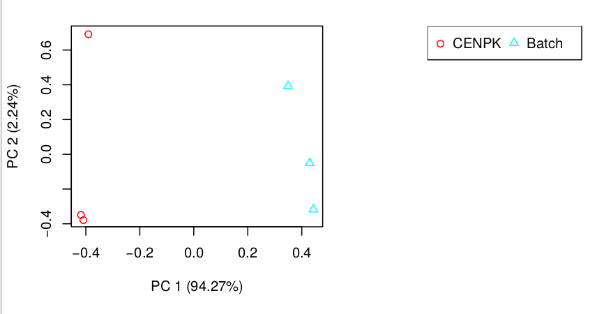
# Another important analysis method to explore relationships among the sample replicates is Principal Component Analysis (PCA). You can generate a PCA plot like so:
$path_to_trinity/Analysis/DifferentialExpression/PtR --matrix kallisto.isoform.counts.matrix --samples design.txt --log2 --min_rowSums 10 --CPM --center_rows --prin_comp 3 - TRANSFERT : Observe plots. Remember, you have to transfert *.pdf files to your home before of transfering into your local machine.
#transfering plots
cp *.pdf /home/formationX/
# from your local machine
scp formationX@YOURADRESSIP:*.pdf .
As you can see in the above, the replicates are more highly correlated within samples than between samples.
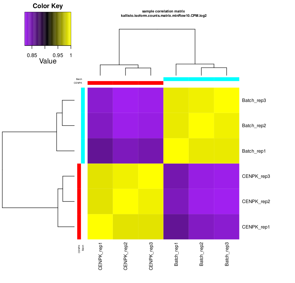
Confirmed by replicate Pearson correlation heatmap:
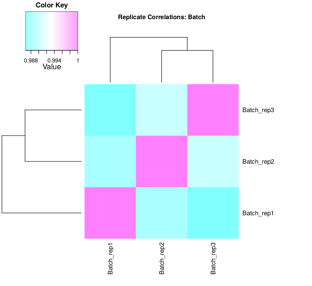
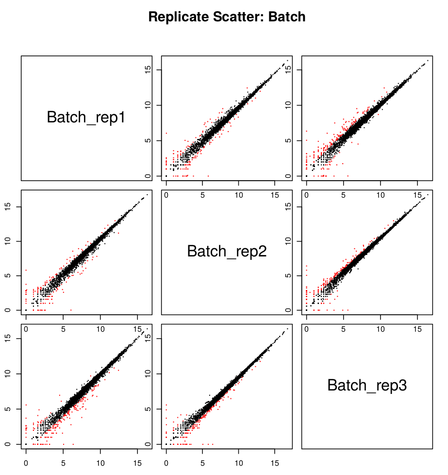
- In this example, the replicates cluster tightly according to sample type, which is very reassuring. If you have replicates that are clear outliers, you might consider removing them from your study as potential confounders.
Results can be also download here
Practice 4 : Mapping against annotated genome reference with Hisat2 + counting with Stringtie

Running Hisat2 and Stringtie with TOGGLe
Connection to account in cluster ssh formationX@YOURIPADRESS
Input data are accessible from :
- Input data : $PATHTODATA/DATA
- Reference : $PATHTODATA/REF/SC_CHR01_genomic.fasta
- Annotation : $PATHTODATA/REF/SC_CHR01_genomic.gtf
- Config file: $PATHTODATA/RNASeqReadCount.config.txt
You can also download from here : RNASeqReadCount.config.txt
Import data from $PATHTODATA to your /scratch/formationX repertory and configure TOGGLe to RNAseq analysis
# Create a TOGGLe-RNASEQ directory in your /scratch
cd /scratch/formationX/
mkdir TOGGLe-RNASEQ
cd TOGGLe-RNASEQ

# Make à copy of the configuration file used by TOGGLe into TOGGLe-RNASEQ directory
scp $PATHTODATA/RNASeqHisat2Stringtie.config.txt .- Change SLURM key
$slurmas below using a texte editor like nanonano RNASeqHisat2Stringtie.config.txtand check the whole of parameters
$slurm
-p YOURPARTITION- in TOGGLe configuration file use /scratch in
$scpkey to launch your job from scratch folder. Your data are now in /scratch so deactivate this option. But activate$envkey usingmodule load TOGGLE/0.3.7module installed on cluster. Check parameters of every step in/scratch/formationX/TOGGLe-RNASeq/RNASeqHisat2Stringtie.config.txtas recommended by https://www.nature.com/articles/nprot.2016.095.
Mapping is performed using HISAT2 and usually the first step, prior to mapping, is to create an index of the reference genome. TOGGle index genome automatically if indexes are absents in reference folder. In order to save some space think to only keep sorted BAM files one these are created. After mapping, assemble the mapped reads into transcripts. StringTie can assemble transcripts with or without annotation, annotation can be helpful when the number of reads for a transcript is too low for an accurate assembly.
[orjuela@node25 orjuela]$ more RNASeqHisat2Stringtie.config.txt
$order
#1=fastqc
2=hisat2
3=samtoolsView
4=samtoolsSort
5=stringtie 1
1000=stringtie 2

$samtoolsview
-b
-h

$samtoolssort

$cleaner
3

# PUT YOUR OWN SLURM CONFIGURATION HERE IF AVAILABLE RESSOURCES
#$slurm
#-p YOURPARTITION

$stringtie 1

$stringtie 2
--merge

$hisat2
--dta

# If your data are in scratch don't activate this option
#$scp
#/scratch/

$env
module load TOGGLE/0.3.7- Now, create a
runTOGGLeRNASEQ.shbash script to launch TOGGLe as follow :
[orjuela@node25 orjuela]$ more runTOGGLe_RNAseq.sh
#!/bin/bash -l
#SBATCH -J TOGGLeRNASeq
#SBATCH --export=ALL
#SBATCH -e toggle."%j".err
#SBATCH -o toggle."%j".out
#SBATCH -p YOURPARTITION

# Defining scratch and destination repertories\n
dir="/scratch/formationX/TOGGLe-RNASEQ/RAWDATA"
out="/scratch/formationX/TOGGLe-RNASEQ/OUT"
config="/scratch/formationX/TOGGLe-RNASEQ/RNASeqHisat2Stringtie.config.txt"
ref="/scratch/formationX/REF/SC_CHR01_genomic.fasta"
gff="/scratch/formationX/REF/SC_CHR01_genomic.gtf"

# Software-specific settings exported to user environment
module load TOGGLE/0.3.7

# running tooglegenerator
toggleGenerator.pl -d $dir -c $config -r $ref -g $gff -o $out --report --nocheck;

echo "FIN de TOGGLe ^^"-
Convert runTOGGLeRNASEQ in an executable file with
chmod +x runTOGGLeRNASEQ.sh -
Launch runTOGGLeRNASEQ.sh in sbatch mode
sbatch ./runTOGGLeRNASEQ.shExplore output OUT TOGGLe and check if everything was ok.
Open and exploreOUT/finalResults/intermediateResults.STRINGTIEMERGE.gtf
[orjuela@node25 OUT]$ more finalResults/intermediateResults.STRINGTIEMERGE.gtf
# /usr/local/stringtie-1.3.4/stringtie /scratch/orjuela/HISAT-STRINGTIE/OUT/output/intermediateResults/0_initialFiles/SRR453566.STRINGTIE.gtf /scratch/orjuela/HISAT-STRINGTIE/OUT/output/intermediateResults/0_init
ialFiles/SRR453567.STRINGTIE.gtf /scratch/orjuela/HISAT-STRINGTIE/OUT/output/intermediateResults/0_initialFiles/SRR453568.STRINGTIE.gtf /scratch/orjuela/HISAT-STRINGTIE/OUT/output/intermediateResults/0_initialFil
es/SRR453569.STRINGTIE.gtf /scratch/orjuela/HISAT-STRINGTIE/OUT/output/intermediateResults/0_initialFiles/SRR453570.STRINGTIE.gtf /scratch/orjuela/HISAT-STRINGTIE/OUT/output/intermediateResults/0_initialFiles/SRR
453571.STRINGTIE.gtf --merge -o /scratch/orjuela/HISAT-STRINGTIE/OUT/output/intermediateResults/1000_stringtie_2/intermediateResults.STRINGTIEMERGE.gtf -G /scratch/orjuela/HISAT-STRINGTIE/REF/GCF_000146045.2_R64_
genomic.gtf
# StringTie version 1.3.4d
NC_001133.9	StringTie	transcript	116	348	1000	.	.	gene_id "MSTRG.1"; transcript_id "MSTRG.1.1";
NC_001133.9	StringTie	exon	116	348	1000	.	.	gene_id "MSTRG.1"; transcript_id "MSTRG.1.1"; exon_number "1";
NC_001133.9	StringTie	transcript	1807	2169	1000	-	.	gene_id "MSTRG.2"; transcript_id "NM_001180043.1"; gene_name "PAU8"; ref_gene_id "YAL068C";
NC_001133.9	StringTie	exon	1807	2169	1000	-	.	gene_id "MSTRG.2"; transcript_id "NM_001180043.1"; exon_number "1"; gene_name "PAU8"; ref_gene_id "YAL068C";
NC_001133.9	StringTie	transcript	2480	2707	1000	+	.	gene_id "MSTRG.3"; transcript_id "NM_001184582.1"; ref_gene_id "YAL067W-A";
NC_001133.9	StringTie	exon	2480	2707	1000	+	.	gene_id "MSTRG.3"; transcript_id "NM_001184582.1"; exon_number "1"; ref_gene_id "YAL067W-A";
Now that we have our assembled transcripts, we can estimate their abundances.
To estimate abundances, we have to run again stringtie using options -B and -e.
prepare data : in a new directory
- Create symbolics links to order data before transfering them to
/scratch
cd /scratch/formationX/TOGGLe-RNASEQ/OUT/
mkdir stringtieEB
cd stringtieEB
ln -s /scratch/formationX/TOGGLe-RNASEQ/OUT/finalResults/intermediateResults.STRINGTIEMERGE.gtf .
ln -s /scratch/formationX/TOGGLe-RNASEQ/OUT/output/*/4_samToolsSort/*SAMTOOLSSORT.bam .
Recovery annotations
- Before merging gtf files obtained by stringtie, we have to recover the annotations in order to see the known genes names in gtf file. Stringtie annotate transcripts using gene id ‘MSTRG.1’ nomenclature . See https://github.com/gpertea/stringtie/issues/179
module load system/python/3.6.5
python3 $PATHTODATA/scripts_utils/gpertea-scripts/mstrg_prep.py intermediateResults.STRINGTIEMERGE.gtf > intermediateResults.STRINGTIEMERGE_prep.gtf
Stringtie -e -B
- Finally, we launch stringtie to obtain de novo transcrits assemblies :
for i in *bam ; do echo "stringtie -e -B over $i ..."; eval "mkdir ${i/.SAMTOOLSSORT.bam/}; module load bioinfo/stringtie/1.3.4; stringtie" $PWD"/"$i "-G $PWD"/"intermediateResults.STRINGTIEMERGE_prep.gtf -e -B -o $PWD/${i/.SAMTOOLSSORT.bam/}/${i/bam/count}"; donegffcompare
- Let’s compare the StringTie transcripts to known transcripts using gffcompare https://github.com/gpertea/gffcompare and explore results. Observe statistics. How many “J”, “U” and “=” do you obtain?.
gffcompare_out.annotated.gtffile will be visualised with IGV later.
$PATHTODATA/scripts_utils/gffcompare/gffcompare -r /scratch/formationX/REF/SC_CHR01_genomic.gtf -o gffcompare_out  intermediateResults.STRINGTIEMERGE.gtf

 /home/orjuela/Documents/2019/BURKINA_FORMATION/TP-OUAGA/REF/SC_CHR01_genomic.gtf  -o gffcompare_out  ../intermediateResults.STRINGTIEMERGE_prep.gtf
  101 reference transcripts loaded.
  6446 query transfrags loaded.
Convert to counts table
- Convert stringtie output in counts using
prepDE.py
# create COUNTS repertory
cd /scratch/formationX/TOGGLe-RNASEQ/OUT
mkdir COUNTS
cd COUNTS/
# create a symbolic link from stringtieEB counts results
ln -s /scratch/formationX/TOGGLe-RNASEQ/OUT/stringtieEB/*/*.count .
# create a GTF list file
for i in *.count; do echo ${i/.SAMTOOLSSORT.count/} $PWD/$i; done > listGTF.txt
Observe the listGTFtxt file :
[orjuela@node25 COUNTS]$ more listGTF.txt
SRR453566 /scratch/formationX/TOGGLe-RNASEQ/OUT/COUNTS/SRR453566.SAMTOOLSSORT.count
SRR453567 /scratch/formationX/TOGGLe-RNASEQ/OUT/COUNTS/SRR453567.SAMTOOLSSORT.count
SRR453568 /scratch/formationX/TOGGLe-RNASEQ/OUT/COUNTS/SRR453568.SAMTOOLSSORT.count
SRR453569 /scratch/formationX/TOGGLe-RNASEQ/OUT/COUNTS/SRR453569.SAMTOOLSSORT.count
SRR453570 /scratch/formationX/TOGGLe-RNASEQ/OUT/COUNTS/SRR453570.SAMTOOLSSORT.count
SRR453571 /scratch/formationX/TOGGLe-RNASEQ/OUT/COUNTS/SRR453571.SAMTOOLSSORT.count- … and launch preDE.py to obtain a global counts file. this global file can be used in DE analysis
python2 $PATHTODATA/scripts_utils/prepDE.py -i listGTF.txt- In this step, you have obtained
gene_count_matrix.csvandtranscript_count_matrix.csvfiles
How many genes have some counts? Remember, we are working only in chr01.
Transfer data from /scratch to your home on cluster
- Don’t forget scp files to your /home/formationX. Transfer reference files fasta, gff and
gffcompare_out.annotated.gtfto use it later with IGV.
# copy gene counts files
scp -r /scratch/SRA_SRS307298/TOGGLe-RNASEQ/COUNTS/*tsv /home/formationX
# copy gffcompare annotation
scp -r /scratch/SRA_SRS307298/TOGGLe-RNASEQ/OUT/stringtieEB/gffcompare_out.annotated.gtf /home/formationX
# copy references
scp -r /scratch/SRA_SRS307298/REF/ /home/formationX
# copy BAMs files but before index it with `samtools index`
for file in /scratch/formationX/TOGGLe-RNASEQ/OUT/output/*/4_samToolsSort/*SAMTOOLSSORT.bam; do samtools index $file; done
# and copy BAM and BAI files
scp /scratch/SRA_SRS307298/TOGGLe-RNASEQ/OUT/output/*/4_samToolsSort/*SAMTOOLSSORT.ba* /home/formationX- Transfert data from your home on cluster to your LOCAL machine (filezilla or scp)
Practice 5 : Visualization of mapped reads against genes using IGV
Practice 5 will be performed with Integrated Genome Viewer (IGV).
Focus on a gene that has been found to be differentially expressed and observe the structure of the gene.
- Run igv :
igv.sh & - Load reference genome, GFF annotation file, BAMs files and the gffCompare
gffcompare_out.annotated.gtfoutput. - Recovery some ID to visualise it in IGV from gffcompare_out.annotated.gtf
orjuela@GFFCOMPARE$ grep  'class_code "u"' gffcompare_out.annotated.gtf | grep ^'NC_001133.9'
NC_001133.9	StringTie	transcript	31192	31470	.	+	.	transcript_id "MSTRG.12.1"; gene_id "MSTRG.12"; xloc "XLOC_000004"; class_code "u"; tss_id "TSS4";
NC_001133.9	StringTie	transcript	151618	152052	.	+	.	transcript_id "MSTRG.75.1"; gene_id "MSTRG.75"; xloc "XLOC_000038"; class_code "u"; tss_id "TSS38";
NC_001133.9	StringTie	transcript	210461	212199	.	+	.	transcript_id "MSTRG.106.1"; gene_id "MSTRG.106"; xloc "XLOC_000055"; class_code "u"; tss_id "TSS55";
NC_001133.9	StringTie	transcript	208135	210131	.	-	.	transcript_id "MSTRG.105.1"; gene_id "MSTRG.105"; xloc "XLOC_000109"; class_code "u"; tss_id "TSS110";
NC_001133.9	StringTie	transcript	28548	28968	.	.	.	transcript_id "MSTRG.11.1"; gene_id "MSTRG.11"; xloc "XLOC_000111"; class_code "u"; tss_id "TSS112";

orjuela@GFFCOMPARE$ grep  'class_code "x"' gffcompare_out.annotated.gtf | grep ^'NC_001133.9'
NC_001133.9	StringTie	transcript	160119	166158	.	+	.	transcript_id "MSTRG.81.2"; gene_id "MSTRG.81"; gene_name "YAR009C"; xloc "XLOC_000042"; cmp_ref "NM_001178213.1"; class_code "x"; tss_id "TSS42";
NC_001133.9	StringTie	transcript	160119	166167	.	+	.	transcript_id "MSTRG.81.1"; gene_id "MSTRG.81"; gene_name "YAR009C"; xloc "XLOC_000042"; cmp_ref "NM_001178213.1"; class_code "x"; tss_id "TSS42";
NC_001133.9	StringTie	transcript	206812	220171	.	-	.	transcript_id "MSTRG.104.1"; gene_id "MSTRG.104"; gene_name "FLO1"; xloc "XLOC_000108"; cmp_ref "NM_001178230.1"; class_code "x"; tss_id "TSS109";

orjuela@GFFCOMPARE$ grep  'class_code "j"' gffcompare_out.annotated.gtf | grep ^'NC_001133.9'
NC_001133.9 StringTie transcript 147594 151166 . - . transcript_id "MSTRG.74.1"; gene_id "MSTRG.74|YAL001C"; gene_name "TFC3"; xloc "XLOC_000096"; cmp_ref "NM_001178148.1"; class_code "j"; tss_id "TSS96";- Search a “unique” gene “MSTRG.12.1” in IGV. Show this loci.
- Search other gene, for example, “MSTRG.81.2” from class “x” or “YAL014C” from class “=”.
6. Differential Expression Analysis (DE) using scripts associated with Trinity software
6.1 Identify differentially expressed genes between the two tissues.
The tool run_DE_analysis.pl is a PERL script that use Bioconductor package edgeR.
# Go to kallisto results
cd /scratch/formationX/KALLISTO
# Run DE analysis
$path_to_trinity/Analysis/DifferentialExpression/run_DE_analysis.pl \
--matrix kallisto_trans.isoform.counts.matrix \
--method edgeR \
--samples_file design.txt \
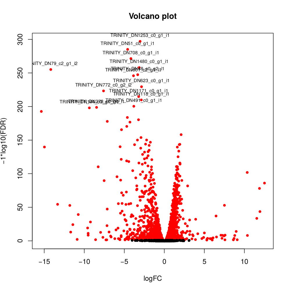
--output edgeR_resultsThe output files are in the directory edgeR_results. Observe file kallisto_trans.isoform.counts.matrix.Batch_vs_CENPK.edgeR.DE_results. It provides several values for each gene:
1) FDR to indicate whether a gene is differentially expressed or not
2) logFC is the log2 transformed fold change between the two tissues
3) logCPM is the log2 transformed normalized read count of average of the samples.
Usually you have to filter this list of genes/isoforms to FDR <0.05 or below. To be more conservative, you could also use more stringent FDR cutoff (e.g. <0.001), and only keep genes with high logFC (e.g. <-2 and >2) and/or high logCPM (e.g. >1). In the edgeR_results directory there is also a “volcano plot” to visualize the distribution of the DE genes.
[orjuela@node25 salmon_outdir]$ head edgeR_results/kallisto_trans.isoform.counts.matrix.Batch_vs_CENPK.edgeR.DE_results
sampleA	sampleB	logFC	logCPM	PValue	FDR
TRINITY_DN332_c0_g1_i10	Batch	CENPK	-10.359903780639	8.33512668205486	0	0
TRINITY_DN730_c0_g2_i1	Batch	CENPK	-6.4740873961699	8.70152404919916	0	0
TRINITY_DN741_c0_g1_i1	Batch	CENPK	-6.31231314146213	10.2830859720565	0	0
TRINITY_DN287_c1_g1_i1	Batch	CENPK	-6.26650019458591	8.47203996977476	0	0
TRINITY_DN65_c0_g1_i3	Batch	CENPK	-4.13189957112457	10.730475730689	0	0
TRINITY_DN1298_c0_g1_i1	Batch	CENPK	-3.19109633696326	8.91247526735535	0	0
TRINITY_DN1253_c0_g1_i1	Batch	CENPK	-3.03997649547823	8.99502681145441	6.47317750883953e-301	3.75444295512693e-298
TRINITY_DN51_c0_g1_i1	Batch	CENPK	-4.59451625218422	10.4521118447878	5.94332889429699e-289	3.01623941385572e-286
TRINITY_DN708_c0_g1_i1	Batch	CENPK	-4.1838974791094	7.70916912374135	3.84699757684993e-275	1.73542335133453e-272
#transfering plots
cd edgeR_result
cp *.pdf /home/formationX/
# from your local machine
scp formationX@YOURADRESSIP:*.pdf .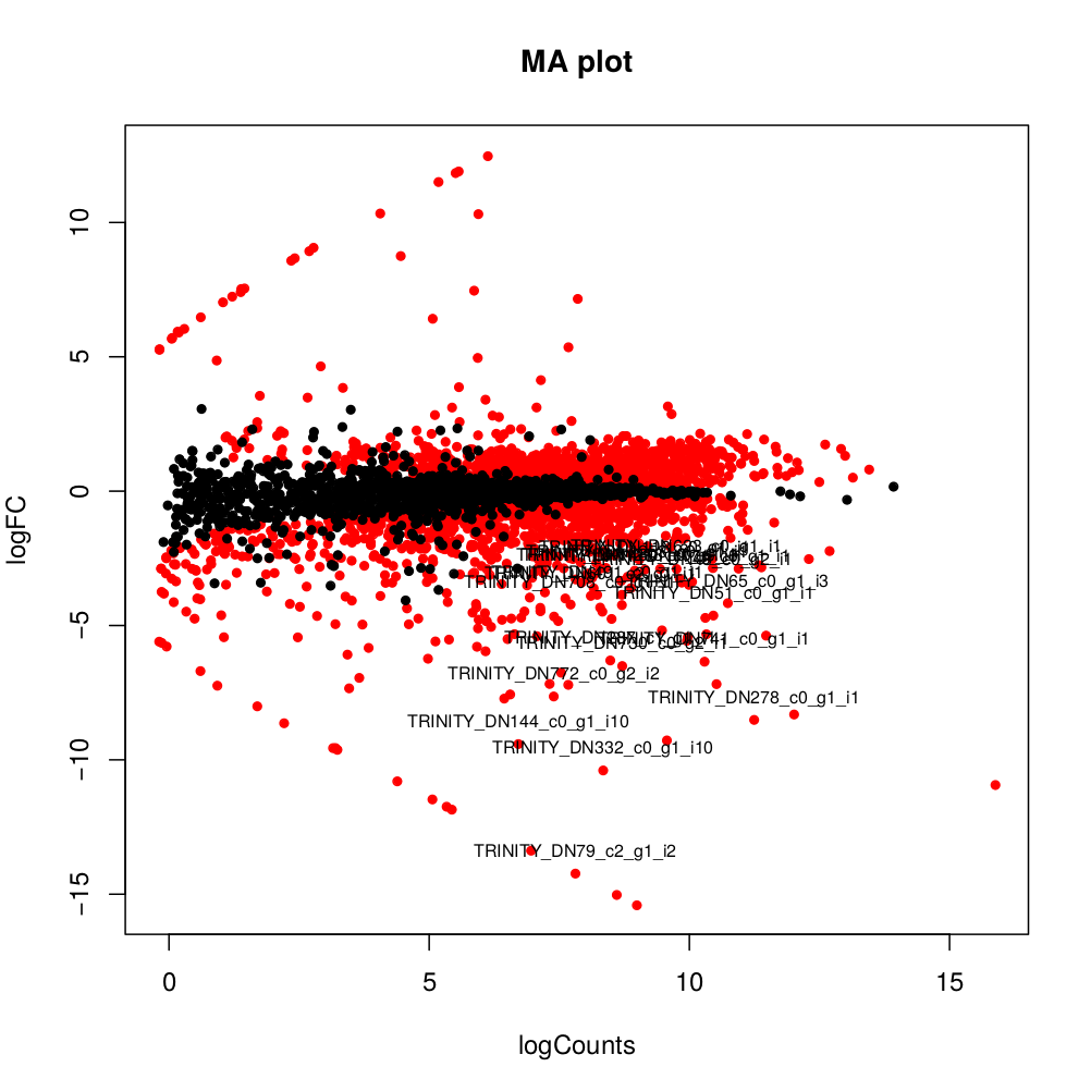
Practice 7 : Differential expression analysis using PIVOT
PIVOT: Platform for Interactive analysis and Visualization Of Transcriptomics data Qin Zhu, Junhyong Kim Lab, University of Pennsylvania Oct 26th, 2017
Intallation of PIVOT
Dependencies that needs to be manually installed. You may need to paste the following code line by line and choose if previously installed packages should be updated (recommended).
install.packages("devtools")
library("devtools")
install.packages("BiocManager")
BiocManager::install("BiocUpgrade")
#BiocManager::install("GO.db")
BiocManager::install("HSMMSingleCell")
#BiocManager::install("org.Mm.eg.db")
#BiocManager::install("org.Hs.eg.db")
BiocManager::install("DESeq2")
BiocManager::install("SingleCellExperiment")
BiocManager::install("scater")
BiocManager::install("monocle")
BiocManager::install("GenomeInfoDb")
Install PIVOT
install_github("qinzhu/PIVOT")
BiocManager::install("BiocGenerics") # You need the latest BiocGenerics >=0.23.3
Launch PIVOT
To run PIVOT, in Rstudio console related to a web shiny interface, use command
library(PIVOT)
pivot()
Go to your web browser.
Introduction
As you have seen, RNA sequencing (RNA-seq) is an experimental method for measuring RNA expression levels via high-throughput sequencing of small adapter-ligated fragments. The number of reads that map to a gene is the proxy for its expression level. There are many steps between receiving the raw reads from the sequencer and gaining biological insight. In this tutorial, we will start with a “Table of counts” and end with a “List of differentially expressed genes”.
Step 1 : Data Input
To input expression matrix, select “Counts Table” as input file type. PIVOT expects the count matrix to have rows as genes and samples as columns. Gene names and sample names should be the first column and the first row, respectively.
- Go to file Tab.
- Take the count file
gene_count_matrix.csvgenerated previously. - Import this file into Data input and then Input file type.
- Add Use Tab separator to Skip Rows.
- Check if yours data are imported in the rigth window.
Step 2 : Input Design Information
The design infomation are used for sample point coloring and differential expression analysis. Users can input the entire sample meta sheet as design information, or manually specify groups or batches for each sample.
- Go to DESIGN.
- Go to Designed Table Upload. Upload
design.txt - Verify that the header of the info file corresponds to the count file.
- Choose the Separator : Space or the appropriate separator.
- Verify on the Design Table Preview and submit design.
- Choose the Normalieation Method :
- for Edge R you can use
DESeq, Trimmed Mean of M-values TMM, or Upperquartile. - for DESeq you can use
DESeq, Modifed DESeq
- for Edge R you can use
In order to have a quick view of your chosen data, look at the summary.
step 3 : Feature Filtering
- There are currently 3 types of feature filter in PIVOT: the expression filter, which filters based on various expression statistics;
- You can choose the filter criteria.
Step 4 : Select samples
- Go To SAMPLE
- Select your sample and condition,
- Subset by sample and or subset by list, as you can create different experiment analysis.
DATA MAP draw a summary of your different analysis, so you can save the history of your analysis.
Step 5 : Basic statistics
- If you want to keep the count table, upload it.
- Check the distribution of each condition in the standard deviation graph, the dispersion graph.
- If needed, you can download the “Variably Expressed Genes”, and on the graph, you can see the dispersion of your data.
First part with EdgeR on PIVOT
- Run the EdgeR program for differential analysis -
EdgeR - Check relevance of normalized expression values provided by EdgeR
- Observe MDS plot of experimental conditions. Observe Smear plot.
Questions :
- Using filters parameters, determine how many genes are found to be differentally expressed using a minimum pvalue <= 0.05, 0.1? Using a minimum FDR-adjusted pvalue <= 0.05, 0.1?
Step 6 : Differential Expression with EdgeR
Once data have been normalized in the Step 1, you can choose the method to find the Differential expression gene between the condition previously choosen. In edgeR, it is recommended to remove genes with very low counts. Remove genes (rows) which have zero counts for all samples from the dge data object.
- Go to Differential Expression, choose edgeR
- According to your normalized method choice in step 1, notify the Data Normalization method, and choose Experiment Design, and condition.
- For this dataset choose
condition, condition - Choose the Test Method, Exact test, GLM likelihood ratio test, and GLM quasi-likelihood F-test.
- For this dataset choose
Exact test
Then Run Modeling
- Choose the P adjustement adapted
- For this dataset choose
False discovery rateorBonferroni correction - Choose FDR cutoff 0.1 and 0.05
- Choose Term 1 and Term 2
You obtain a table containing the list of the differential gene expressed according to your designed analysis. This table contains logFoldChange, logCountPerMillion, PValue, FDR. This table can be download in order to use it for other analysis. The Mean-Difference Plot show you the up-regulated gene in green, and Down regulated gene in black.
- Keep this file
edgeR_results.csv - Change the name of the file according to your analysis.
- Example :
edgeR_results_FDR_01.csvto be able to recognize the different criteria used.
Questions :
- Do you have the sample number of differential gene for a FDR cutoff 0.1 and 0.05?
- According to you, what is the best cutoff?
- When you change the order of the Term1 and Term2, what are the consequences on the Results Table?
Second part with DESeq2 on PIVOT
- Run the DESeq program for differential analysis -
DESeq2 - Check relevance of normalized expression values provided by DESeq2
- Observe MDS plot of experimental conditions. Observe Smear plot.
Questions:
- Using filters parameters, determine how many genes are found to be differentially expressed using a minimum pvalue <= 0.05, 0.1? Using a minimum FDR-adjusted pvalue <= 0.05, 0.1?
Step 6 : Differential Expression with DESeq2
Once data have been normalized in the Step 1, you can choose the method to find the Differential expression gene between the condition previously choosen.
- Go to Differential Expression, choose DEseq2
- According to your normalized method choice in step 1, notify the Data Normalization method, and choose Experiment Design, and condition.
- For this dataset choose
condition, condition - Choose the Test Method, Exact test, GLM likelihood ratio test, and GLM quasi-likelihood F-test.
- For this dataset choose
Exact test
Then Run Modeling
- Choose the P adjustement adapted
- For this dataset choose
FDR cutoff - Choose FDR cutoff 0.1 and 0.05
You obtain a table containing the list of the differential gene expressed according to your designed analysis. This table contains baseMean, log2FoldChange, PValue, pvalueadjust. This table can be downloaded in order to use it for other analysis. The MA Plot show you the up-regulated gene LFC>0, and Down regulated gene LFC<0, the differential gene are in red.
- Keep this file
deseq_results.csv - Change the name of the file according to your analysis.
- Example :
deseq_results_FDR_01.csvto be able to recognize the different criteria used.
Questions :
- Do you have the sample number of defferential gene for a FDR cutoff 0.1 and 0.05?
- According to you, what is the best cutoff?
- When you change the order of the Term1 and Term2, what are the consequence on the Results Table?
Step 7 : Visualisation Heatmap, Correlation, PCA
You can make correlation between the control and the rep in order to identify library bias if exists. We can also explore the relationships between the samples by visualizing a heatmap of the correlation matrix. The heatmap result corresponds to what we know about the data set. First, the samples in group 1 and 2 come from the control and the repetition, so the two groups are very different. Second, since the samples in each group are technical replicates, the within group variance is very low.
Correlation between sample and control
- Go to Correlation.
- 1 Pairwaise Scatterplot show the pairwaise comparison between your samples.
- 2 Sample correlation with 3 methods, pearson, sperman or kendal, with the agglomeration method show you how are linked your samples.
- 3 Feature Correlation represented with a heatMap ordered by variance of the expression.
PCA
- To separate your sample a PCA is way to make a dimension reduction.
Question :
- Can you describe the structure of your sample, with a correlation analysis, and a PCA?
Practice 8 : Compare list of DE genes with EdgeR and DESeq2
Practice 8 will be performed with Venn Diagramm implemented on PIVOT.
- Compare lists of DE genes with the two approches.
- Go to Toolkit.
- Upload your lists of gene obtained with edegR
edgeR_results_FDR_01.csv, and DESeq2deseq_results_FDR_01.csv. - Upload the first list then Add List and upload the second list.
- You can see the Venn diagram and download the common list of gene between the both methods.
Questions:
- Look at the expression values for a gene found DE with EdgeR and not with DESeq2, and vice-versa, give the pvalue of each gene?
Some other tools are available to compare 2 lists of gene. Venny.
Practice 9 : Hierarchical Clustering
Practice 9 will be performed with PIVOT.
- Connect to your PIVOT interface.
- Go to Clustering.
- For each analysis EdgeR or DESeq2 specify the Data Input (count, log…).
- Choose the distance
Euclideanor an other, the Agglomeration methodWardand the number of cluster.
Links
- Related courses : Transcriptomics
- Degust : Degust
- MeV: MeV
- MicroScope: MicroScope
- Comparison of methods for differential expression: Report
- PIVOT: PIVOTGithub
- DESeq2: DESeq2
- EdgR: EdgeR
License
